
The data cell display is limited by the physical size of the cell at the time the user is working with the spreadsheet. You may notice that if the cell size is too small, the display changes to a series of hash-marks, indicating that the available space is too small to display a meaningful value.
When we perform numerical calculations the desired accuracy depends on the problem we are solving. You know from buying gasoline, that even though the prices are quoted as $3.6999, you always pay the amount rounded to the nearest cent. At other times, we wish to perform the computation as accurately as possible.
Excel application provides us with two ways of adjusting the display of numerical data. The first one is through formatting. The Number menu in the Home toolbar allows us to select the number of decimal digits that will be displayed, and to choose whether the numerical data represents currency, time, date, percentage, etc. We will explore the properties of some of these data formats.
The second way is to define the appropriate format for the cell by selecting a specific format. The effect of selecting the format is that the value that the cell represents assumes to be the value that is displayed. Let us see on a concrete example what does this mean.
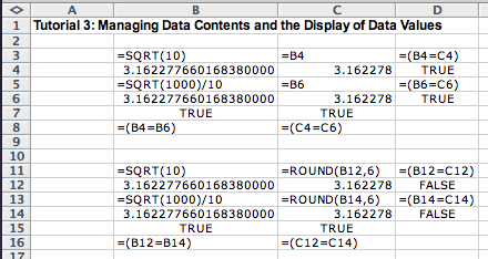
We set up a simple example. The value of the cell B4 is computed to be the square root of 10:

We change the width of the column B and increase the number of decimal
points that are displayed by clicking on the Increase Decimal
tab in the Number part of teh Home toolbar. For
comparison we also include the result of the formula
=SQRT(1000)/10 --- that should evaluate to the same
number. We notice, that all digits beyond 15 significant digits are
zeros, regardless of how many decimal digits we choose to display. The
computer limits the size of all numbers, unless the programmer takes
extraordinary measures to preserve higher accuracy. To do so is beyond
the study of introductory computing. However, we wish to see whether
these two values, computed in a slightly different way, are considered
to be the same. We copy the two values to the adjacent column C and
then run some tests. Each comparison is defined as shown above for the
cells D4 and D6, or below for the cells B7 and B8. We see that
regardless of teh data representation, the values are considered to be
the same.

We now copy the cells below, but change the values in the cells B12 ans B14 to be rounded to six decimal digits. We see that while the displayed values are the same the comparison of the original value and the rounded value fails. We need to keep this in mind when designing programs. We must consider in each case wehther we want to retain the original accuracy of the computation or whether we want to round the value to a specific number of decimal digits.
We will now consider the ways in which the Excel application orders different types of data. If we know how to compare two data values and decides which one is smaller and which one is larger, or which one comes first (e.g. a word in a dictionary) and which comes later, we can arrange a list of data in a sorted order. We can also find the smallest value or the largest value.
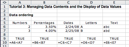
Let us look at some of the data types for which Excel can determine the order. These are numbers, percentages, dates, letters, and text. Here are some examples with the comparisons to verify that Excel does understand the ordering:
For some of the data types the Excel also knows how to compute the next value. If our list of data starts with the numbers 1 and 2, we can extend the numbers to a list of numbers 1, 2, 3, 4, ... by highlighting the adjacent cells that contain 1 and 2 and dragging the (invisible) successor formula to the remaining cells. Let us see what happens if we try to extend our original data to the cells below in this manner:
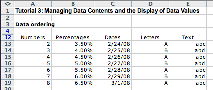
We see that not only can Excel find a succcessor for numbers, it also
determines the next percentage by replicating the difference
between the first two values. It also correctly find the next
date, including the knowledge of leap years. However, it does
not know what is the next letter in a sequence that starts with
A and B, and so when we try to extend these
two values, it just repeats the pattern there. The same happens with
the text in the cells E12 and E13.
We have already seen in our early examples that Excel defines
functions that can find the minimum and the maximum values in a list
of numbers, can compute the average, median, and other statistical
function over numerical data. Let us see whether we can apply the
MIN and MAX functions to values of types
other than plain numeric data type:
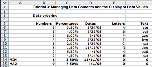
The example shows that we can find the minimum or maximum
date and percentage values, but we get a
nonsense value, just number 0, when we try to find the minimum or the
maximum value among letters or text type of data values.
However, we can sort the data so that the list is ordered either in the ascending order or in the descending order. This is such a fundamental operation that it appears as a separate entry in the Editing tab of the Home toolbar. It is not entered as a function. Instead, we select the list of data to sort and apply the sort operation to that list. The values in the cells in the selected list change so that they are now in the sorted order. We first show how each of our lists of data changes when we sort it in ascending order:
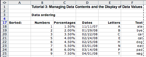
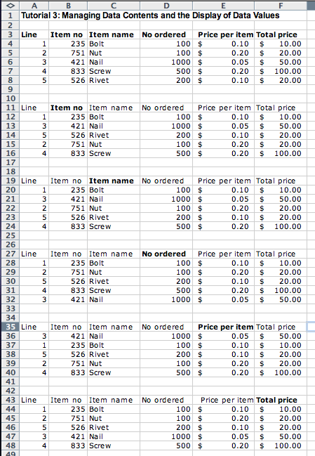
We had to fight Excel a bit when applying sorting to our selected data --- it kept asking us whether the data in adjacent columns should be included in sorting. The reason for doing this is that typically several adjacent columns represent information about one data object. In the following example we have five lines in an invoice, each representing the ordering of one kind of item:

We select the entire order and decide to sort it. Select the
Practice these skills and explore the Excel behavior on the following problems:
MONTH and DAY functions. Now sort
the data first by month then by day. In the Sort dialog
choose Add Level then instruct the sorting to be done first
by months, then by days.